Day 1: Basics of R
Department of Applied Economics, University of Minnesota
Slide Guide
- Click on the three horizontally stacked lines at the bottom left corner of the slide, then you will see the table of contents, and you can jump to the section you want to see.
- Hitting letter “o” on your keyboard and you will have a panel view of all the slides.
- You can directly write and run R code, and see the output on slides.
- When you want to execute (run) code, hit
command+enter(Mac) orControl+enter(Windows) on your keyboard. Alternatively, you can click the “Run Code” button on the top left corner of the code chunk.
Learning Objectives
- To understand the R coding rules.
- To understand the basic types of data and structure in R, and to be able to manipulate them.
- To be able to use base R functions to do some mathematical calculations.
- To be able to create R projects and save and load data in R.
Reference
Today ’s outline
Before you start
Note
- We’ll cover many basic topics today.
- You don’t need to memorize nor completely understand all the contents in this lecture.
- At the end of each section, I included a summary of the key points you need to know. As long as you understand those key points, you are good to go.
General coding rules in R
General coding rules in R
Rules
R programming language is object-oriented programming (OOP), which basically means: “Everything is an object and everything has a name.”
-
You can assign information (numbers, character, data) to an object with
<-or=(e.g.,object_name <- value) and reuse it later.- e.g
x <- 1assigns 1 to an object calledx.
- e.g
If you assign information to an object of the same name you already used, the object that had the same name will be overwritten.
Once objects are created, you can evaluate them to see what’s inside.
Example
Rules
- You can name the object whatever you want, but it must start with a letter.
- You can use
_or.in the object name. - It is recommended to use a meaningful name for the object so that you can understand what the object contains.
Rules
R has a lot of packages that provide additional functions and data. To use the functions in the package:
You need to install the package with
install.packages("package_name"). (You need to do this only once.)Whenever you want to use the functions in the package in the current R session, you need to load the package with
library(package_name).
- You’ll get an error message like
could not find function "xxxx"if you forget to load the package.
Basic data types (i.e., atomic data types) in R
Overview
These are the basic data elements in R.
| Data Type | Description | Example |
|---|---|---|
| numeric | General number, can be integer or decimal. |
5.2, 3L (the L makes it integer) |
| character | Text or string data. | "Hello, R!" |
| logical | Boolean values. |
TRUE, FALSE
|
| integer | Whole numbers. |
2L, 100L
|
| complex | Numbers with real and imaginary parts. | 3 + 2i |
| raw | Raw bytes. | charToRaw("Hello") |
| factor | Categorical data. Can have ordered and unordered categories. | factor(c("low", "high", "medium")) |
Note
- Don’t worry about the details. numeric , character, and logical are the most common data types you will see in R.
- If you use character type, you alway need to put the text in either single quotes (’) or double quotes (“).
Use class() or is.XXX() to examine the data types.
You can convert one type of data to another type of data using the as.XXX() function.
Three conversion functions that are used often are:
Logical values (a.k.a. Boolean values) (important)
Rules
- A Logical values are
TRUE,FALSE(andNA, which means “not available” or “undefined value”). - Logical values are often results of comparison operations such as
<(less than),>(greater than),<=(less-than-or-equal),>=(greater-than-or-equal),==(equal), and!=(not-equal). - As we will see later, a sequence of logical values (i.e., logical vectors) can be used as an index vector to subset the data.
- When a logical value is used like numeric,
TRUEis treated as 1 andFALSEis treated as 0.
- Relational operators (or comparison operator):
==,!=,>,<,>=,<=. - Logical operators:
&(and),|(or), and!(not).
Key points
At this point,
- There are specific definitions of data types in R.
- Specifically, “numeric”, “character”, “logical” are popular.
- You can check the data type using
class()function. - You can convert one data type to another using
as.XXX()function. - Remember that logical values can play some important roles in R.
Types of Data Structures in R
Types of Data Structures in R
Depending on how the data is stored, R has several types of data structures.
| Data Structure | Description | Creation Function | Example |
|---|---|---|---|
| Vector | One-dimensional; Holds elements of the same type. | c() |
c(1, 2, 3, 4) |
| Matrix | Two-dimensional; Holds elements of the same type. | matrix() |
matrix(1:4, ncol=2) |
| Array | Multi-dimensional; Holds elements of the same type. | array() |
array(c(1:12), dim = c(2, 3, 2)) |
| List | Can hold elements of different types. | list() |
list(name="John", age=30, scores=c(85, 90, 92)) |
| Data Frame | Like a table; Each column can hold different data types. This is the common data structure. | data.frame() |
data.frame(name=c("John", "Jane"), age=c(30, 25)) |
Note
Here, we focus on how to create and how to use each of the data structures.
Vector (one-dimensional array)
Vector: How to Manipulate?
Basics
You can retrieve single or multiple elements of a vector by indexing with
[]brackets. Inside[], you simply provide another vector containing the position of the element you want to extract.If a vector has names, you can also use the name of the element to extract it.
To modify a specific element, you can assign a new value to the position you want to modify.
Example
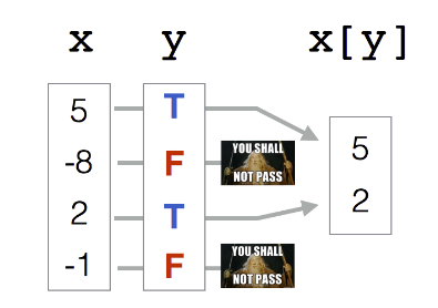
- A logical vector is a vector that only contains logical values (TRUE and FALSE values).
- You can use a logical vector as an index vector to subset elements of the vector. Only the elements that correspond to TRUE values are returned.
Example
The following figure explains the mechanism of logical indexing.
Exercise
The following code randomly samples 30 numbers from a uniform distribution between 0 and 1, and stores the result in x.
Questions
- Extract the 10th and the 15th elements of
x. - Extract elements larger than \(0.5\).
- Replace the 10th and the 15th elements of
xto 0. - If an element of
xis larger than \(0.9\), replace it with \(1\). - Count the elements larger than \(0.6\).
Matrix (Two-dimensional array)
- A matrix is a collection of elements of the same data type. It consists of rows and columns. (It’s essentially a vector with an additional dimension attribute.)
- I haven’t seen a matrix data structure in real-world data. It is mainly used for linear algebra operations.
-
matrix()function is used to create a matrix.
Syntax
Note
- You need to specify the
vector_dataand thenumber_of_rowsandnumber_of_columns. - If the length of
vector_datais a multiple ofnumber_of_columns(ornumber_of_rows), R will automatically figure how many rows (or columns) are needed. - As an option, you can specify
byrow = TRUEto fill the matrix by row. By default, the value invector_datais filled by column.
Matrix: How to Manipulate
Again, you can access the elements of a matrix using [] brackets. But now you have options to specify the row and column index.
Example
You can add column names and row names to a matrix using colnames() and rownames() functions. If a matrix has column names and row names, you can use the names as the index.
Matrix: Exercise Problem (Optional)
Use the following matrix:
- Extract the element in the 2nd row and 3rd column.
- Extract the 2nd row.
- Subset the rows where column “A” is larger than 0.5. (Use logical indexing).
Data Frame
-
data.frameclass object is like a matrix but it can store any type of data in each column. - It is optimized for tabular data. That’s why we see this data structure in the real-world data.
Syntax
Example
If column names are not provided, R will assign column names to those columns automatically.
Again, you can access the elements of a data.frame using [ ] (brackets) operator. But you need to specify the row and column index like you did in the matrix.
As an index vector, you can use a vector of logical values, column names, and positional index.
You can also extract specific column values using $ or [[ ]] operator.
$and[[ ]]can only select a single column and return as a vector, whereas[ ]can select multiple columns ((see?"$",?"["and?"[["about the difference in those operators).Inside
[[ ]]you provide the column name as a character.Why do we need this? As you’ll see later, vector data is the most common input data structure when doing basic linear algebra in R (mean, sum, sqrt, etc.). (and it’s the fastest way to do the calculation in R!)
You can add a new column to a data.frame object using the $ operator.
Syntax
-
vector_datato be added must have the same length as the number of rows in the data.frame, otherwise the value is recycled.
Exercise Problem
We will use the built-in dataset mtcars for this exercise. Run the following code to load the data.
Extract the rows corresponding to the cars with the row numbers 1, 5, and 10 using numeric indexing
Add a new column to the
mtcarsdata frame calledpower_to_weight_ratio, which is calculated as the ratio of horsepower (hp) to weight (wt).Create a new data frame called
efficient_carsthat contains cars withmpggreater than20and power-to-weight ratio less than 5.(Optional) Sort the efficient_cars data frame by the
power_to_weight_ratiocolumn in ascending order and display the result. [Hints: (1)useorder()function to sort the data frame. (2) Useorder(efficient_cars$power_to_weight_ratio)as an index vector.]
with() and within()
with() and within() functions are useful when you want to do some operation on a data.frame.
with(data_frame, function(column1))function allows you to evaluate an expression in the context of adata.frame.within()function is similar towith(), but it allows you to modify thedata.framein place.
With these functions, you can avoid typing the data frame name and $ mark, repeatedly.
Example
List
A list in R can store elements of different types and sizes, including numbers, characters, vectors, matrices, data frames, and even other lists.
A
listis a collection of data that can have any data and data structure type as its element. You can create a list usinglist()function.
You can access list elements using $ amd [ ] or [[ ]] brackets.
- The
[ ]operator returns a list of the selected elements. - The
[[ ]]and$operators return any single element as it is.$can be used only when the list has names.
Summary
Here are the key points I want you to know:
Key Points
- To know how to create
vector,matrix,data.frame, andlistin R.- Vector and matrix stores the same data type, whereas data.frame and list can store different types of data.
- To access and subset and modify the elements of the object, use indexing (logical, positional, and named).
- For indexing, you can use
[ ],$, and[[ ]]operators.
- For indexing, you can use
Matrix/Linear Algebra in R
For the calculation of remainder and quotient, you don’t need to remember the operator.
Arithmetic operations of vectors are performed by element-wise (element by element in the same position).
If you want to do matrix multiplication, you need to use %*% operator. Otherwise, it will be element-wise multiplication.
Loading and Saving Data in R
R base functions for data import and export
- Like other softwares (e.g., Stata, Excel) do, R has two native data formats:
.Rdata(or.rdata) and.Rds(or.rds)-
.Rdatais used to save multiple R objects, -
.Rdsis used to save a single R object
-
.Rdata format
- Load data:
load("path_to_Rdata_file")
- Save data:
save(object_name, file = "path_to_Rdata_file")
.Rds format
- Load data:
readRDS("path_to_Rds_file")
- Save data:
saveRDS(object_name, file = "path_to_Rds_file")
Setting the working directory
To access to the data file, you need to provide the path to the file (the location of the data file).
Example
Suppose that I want to load flight.rds in the Data folder. On my computer, the full path (i.e., absolute path) to the file is /Users/shunkeikakimoto/Dropbox/git/R_summer_2024/Data/flight.rds.
Problems
- I do not want to type the full path every time I load the data. It’s too cumbersome.
- If you are working with a team, your code might not work for other person because the path to the data file is different for each people.
-
Working Directory is a file path on your computer where R looks for files that you ask it to load, and where it will put any files that you ask it to save.
- You can check the current working directory using
getwd()function. - By default, R (
.Rfile) uses your home directory as the working directory.
- You can check the current working directory using
- If you expect to import and/or export (save) datasets and R objects often in that particular directory, it would be nice to tell R to look for files in the directory by default.
- You can use
setwd()to designate a directory as the working directory:
Example 1
In my case, I set the working directory to the Data folder.
Now, R will look for the data file in the Data folder by default. So, I can load the data using relative path, not absolute path.
Problems
- Still,
setwd()relies on an absolute file path, which might vary by person (e.g., some person save folder in Dropbox, other person uses Google Drive). - So, designating working directory using
setwd()does not solve the second problem completely (i.e, If you are working with a team, the path to the data file is different for each person.)
“R experts keep all the files associated with a project together — input data, R scripts, analytical results, figures. This is such a wise and common practice that RStudio has built-in support for this via projects.” - R for Data Science Ch 8.4
RStudio Projects
An RStudio project is a way to organize your work.
Once an R project is loaded, it automatically sets current working directory to the folder where that
.Rprojfile is saved (you don’t need to usesetwd()!).As long as the folder structure in the project folder is the same (relative path from the folder containing
.Rprojfile), you can share the code involving data loading with your team members.
Follow this steps illustrated in this document: R for Data Science Ch 8.4
- On your Rstudio, check the top-right corner of the Rstudio window. You will see the name of the project you created.
- Alternatively, you can open the project by clicking the
.Rprojfile via Finder (Mac) or File Explorer (Windows).
- Alternatively, you can open the project by clicking the
- Now, let’s check the current working directory using
getwd()function. You will see the path to the project folder. - Let’s load
flight.rdsdata file withreadRDS()function.
Loading data other than .Rds (.rds) format
- R can load data from various formats including
.csv,.xls(x), and.dta. - There exists many functions that can help you to load data:
-
read.csv()to read a.csvfile -
read_excel()from thereadxlpackage to read data sheets from an.xls(x)file -
read.dta13()function from thereadstata13package to read a STATA data file (.dta)
-
Use import() function of the rio package
-
But
import()function from theriopackage might be the most convenient one to load various format of data.- Unlike,
read.csv()andread.dta13()which specialize in reading a specific type of file,import()can load data from various sources.
- Unlike,
In Data folder, flight data is saved with three different formats: flight.csv, flight.dta, and flight.xlsx. Let’s load the data using import() function on your Rstudio.
Saving the data
- You can save the data with various formats.
-
But, unless necessary, it is recommended to save the data in
.rdsformat.- how?:
saveRDS(object_name, path_to_save)
- how?:
Reasons + If you work with R, there is no reason to save the data in other formats than .rds. + .rds format is more efficient in terms of saving and loading the data. + Check the size of the flight data files in different formats. Which one is the smallest?
Let’s try!
- Load the
flightdata in theDatafolder.
Summary
Important
- Rstudio project (
.Rproj) is a useful tool to organize your work. As long as the folder structure under the.Rprojis the same, you can share the code involving data loading with your team members. - To load data:
- use
readRDS()function for.Rds(.rds) format. - you can use
import()function from theriopackage for various format.
- use
- To save the data, it is recommended to use
.rdsformat and usesaveRDS()function.
Exercise Problems
Exercise Problems 1: Vector
Create a sequence of numbers from 20 to 50 and name it
x. Let’s change the numbers that are multiples of 3 to 0.sample()is commonly used in Monte Carlo simulation in econometrics. Run the following code to creater. What does it do? Use?sampleto find out what the function does.
- Find the value of mean and SD of vector
rwithout usingmean()andsd() - Figure out which position contains the maximum value of vector
r. (usewhich()function. Run?which()to find out what the function does.) - Extract the values of
rthat are larger than 50. - Extract the values of
rthat are larger than 40 and smaller than 60. - Extract the values of
rthat are smaller than 20 or larger than 70.
Exercise Problem 2: Data Frame
- Load the file
nscg17small.dta. You can find the data in theDatafolder.- This data is a subset of the National Survey of College Graduates (NSCG) 2017, which collects data on the educational and occupational characteristics of college graduates in the United States.
- Each row corresponds to a unique respondent. Let’s create a new column called “ID”. There are various ways to create an ID column. Here, let’s create an ID column that starts from 1 and increments by 1 for each row.
- To take a quick look at the summary statistics of a specific column,
summary()function is useful. Usesummary()to create a table of the descriptive statistics for salary. You’ll provide salary column tosummary()as a vector. - Create a new variable in your data that represents the z-score of the hours worked (use
hrswkvariable). \[Z = (x - \mu)/\sigma\] , where \(Z = \text{standard score}\), \(x =\text{observed value}\), \(\mu = \text{mean of sample}\), and \(\sigma = \text{standard deviation of the sample}\). - Calculate the share of observations in your data sample with above average hours worked.
Appendix: A List of Useful R Built-in Functions
| Function | Description |
|---|---|
length() |
get the length of the vector and list object |
nrow(),ncol()
|
get the number of rows or columns |
dim() |
get the dimension of the data |
rbind(),cbind()
|
Combine R Objects by rows or columns |
colMeans(), rowMeans()
|
calculate the mean of each column or row |
with and within()
|
You don’t need to use $ every time you access to the column of the data.frame. |
ifelse() |
create a binary variable |
paste(), paste0()
|
concatenate strings |
| Function | Description |
|---|---|
sum(), mean(), var(), sd(), cov(), cor(), max(), min(), abs(), round() |
|
log() and exp()
|
Logarithms and Exponentials |
sqrt() |
Computes the square root of the specified float value. |
seq() |
Generate a sequence of numbers |
sample() |
randomly sample from a vector |
rnorm() |
generate random numbers from normal distribution |
runif() |
generate random numbers from uniform distribution |