Rmarkdown for making a PDF document

This section briefly introduces Rmarkdown, a simple tool to blend text, code, and output in one file. It lets you create summary reports, presentation slides, dashboards, and more. We’ll look at creating a PDF document as an example, but you can use the same steps for HTML and other formats. The following section will cover Quarto, an improved version of R Markdown. Once you’re familiar with Rmarkdown, you’ll find Quarto easy to use.

Before Starting

If you have not installed Rmarkdown package, install it by running install.packages("rmarkdown").
Make sure that your computer has a LaTeX distribution installed. You can download and install the TinyTeX distribution with the R package tinytex. Unlike other LaTex distributions like MacTeX, tinytex is a lightweight distribution that only includes the essential packages needed to render R Markdown documents to PDF.

tinytex::install_tinytex()
# to uninstall TinyTeX, run
# tinytex::uninstall_tinytex()

Reference: “R Markdown Cookbook” by Yihui Xie, Christophe Dervieux, and Emily Riederer [here]

1. Getting Started

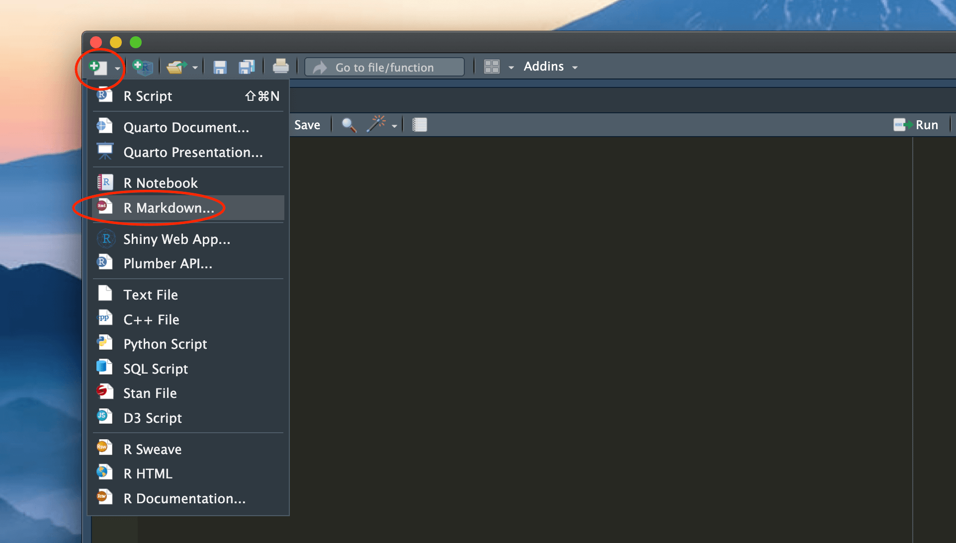
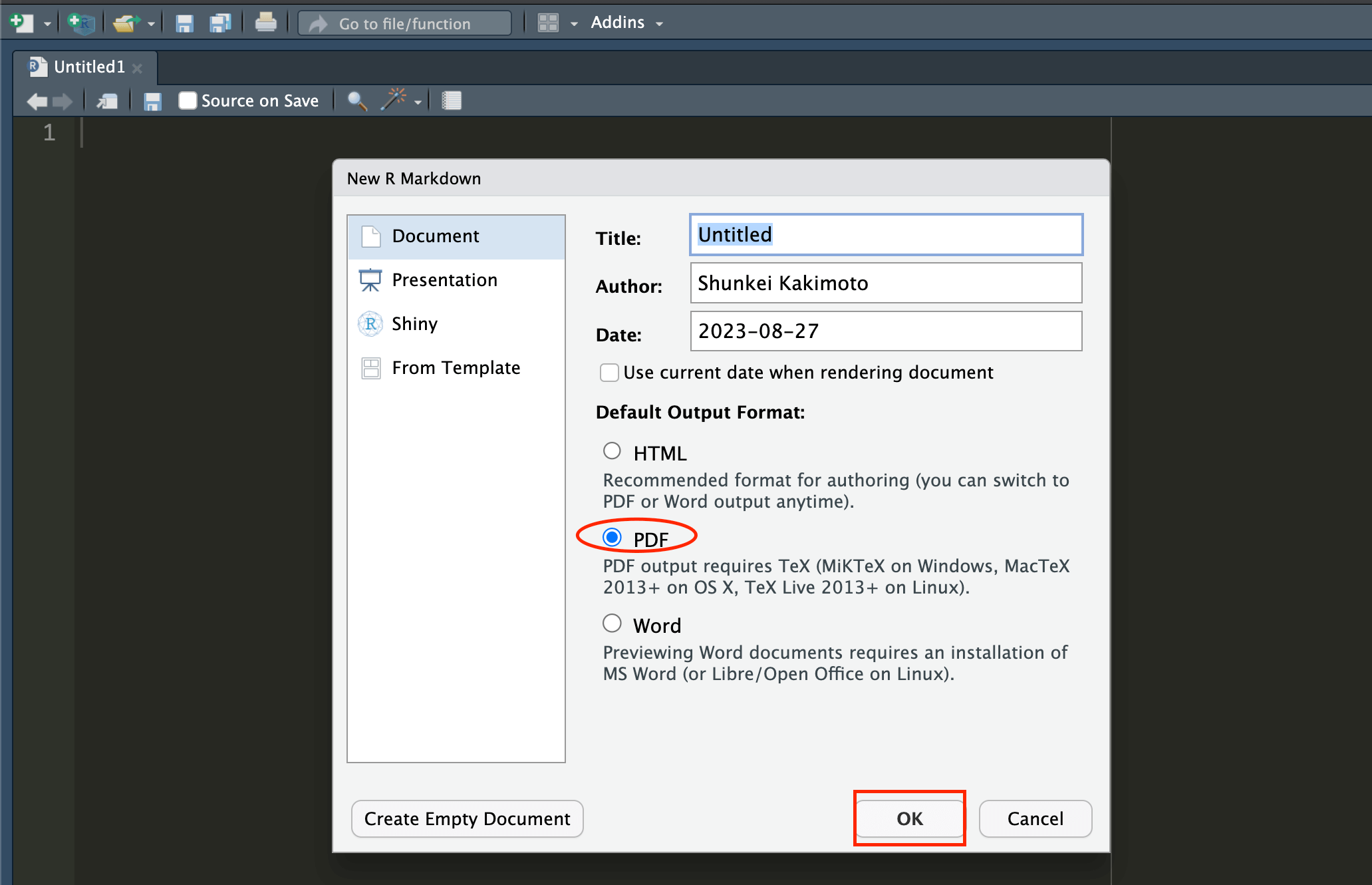
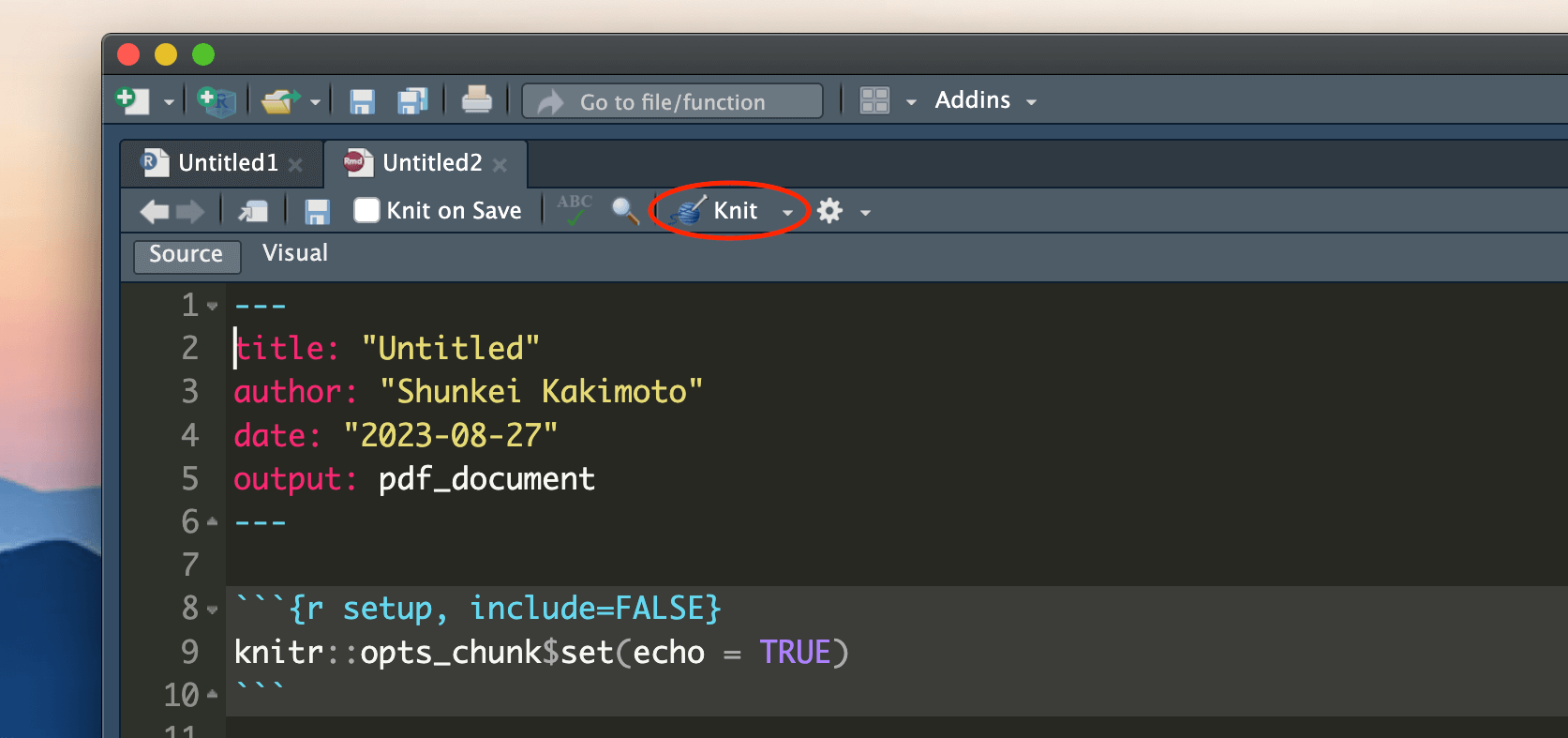
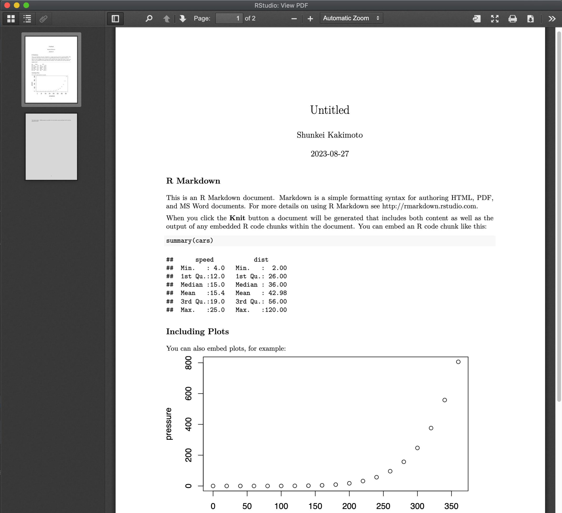
From top-down of New file icon, crick “R Markdown” -> Select “PDF” format -> A new Rmarkdown (.Rmd) file pops up -> Crick “Knit” bottom to run the Rmd file.

Step 2: You can choose HTML if you want a HTML document.

2. Basic Components of Rmarkdown

An R Markdown document is divided into three main parts:

YAML header
text body
code chunks.

Let’s take a closer look at each of these components briefly.

YAML Header

The Rmarkdown document starts with a YAML header. It is a set of key:value pairs bounded by triple dashes ---. It contains metadata about the document, such as the title, author, and output format. Here is an example of a YAML header:

---
title: "My Document"
author: "Your Name"
date: "2022-10-10"
output: pdf_document
---

In the output option, you can specify the document’s output format. For example, output: pdf_document will render the document as a PDF file. Other options include output: html_document for an HTML file and word_document for a Word document¹. You can further customize the output format by adding additional options. For example, pdf_document has options such as toc for a table of contents and number_sections to number the sections.

---
title: "My Document"
author: "Your Name"
date: "2022-10-10"
output:
  pdf_document:
    toc: true
    number_sections: true
---

Markdown Syntax

Ramrkdown and Quarto use Markdown syntax to format text. These are just some rules for formatting texts (e.g., how to make a header, how to make a font bold or italic, how to make a list, etc.). Check this document to see how to use Markdown syntax to syle your texts: Markdown Basics..

Code Chunks

In R Markdown document, you write R code in a block called a code chunk. It looks like this:

```{r}
print("Hello, World!")
```

There are many options you can configure for code chunks. For more detailed information about chunk options, please refer to this article. Chunk options are specified in the body of a code chunk after #| (you can also define chunk options inside the curly braces ```{r}, but Quarto utilizes #| for setting chunk options. To ensure consistency in syntax between Rmarkdown and Quarto documents, it is advisable to use #|).

For example, you can hide the code from the final document by setting echo: false:

```{r, summary-pressure}
#| echo: false
summary(pressure)
```

You can name the code chunk inside the ```{r}. This is useful for several reasons. For example, if error happens in the code chunk when rendering the document, you can easily locate the code chunk that caused the error because R Markdown will display the label of the code chunk in the error message. Also, if you want to cross-reference a figure or table in the text, you can use the label of the code chunk².

Here is another example of a code chunk that generates a figure. In this case, the code chunk is labeled fig-pressure, and the figure caption is set to “A figure caption”. The width of the figure is set to 50% of the width of the image container.

```{r, fig-pressure}
#| fig.cap: "A figure caption"
#| out.width: 50%

plot(pressure)
```

Although the base rmarkdown package does not provide direct support for cross-referencing, if you are using the bookdown package and setting output: bookdown::pdf_document2 or/and output: bookdown::html_document2 in the YAML header, you can use the make cross-reference figures and tables using the syntax @ref(type:label). For example, if you want to refer to a figure with the label fig-pressure, you can refer the figure with @ref(fig:fig-pressure). Try it on your Rmarkdown document!. For more detailed information about cross-referencing, please refer to this document.

Global Options

Instead of manually setting the same chunk options in every code chunk (e.g., figure size), you can configure the default options for all code chunks in the document using the knitr::opts_chunk$set() function ( opts_chunk$set() function of the knitr package). For example, you can set the default figure size and alignment like this:

```{r, setup}
#| include: false

knitr::opts_chunk$set(
  fig.width = 6, 
  fig.height = 4,
  fig.align = "center"
)
```

include: false means that the code and results associated with this chunk will not be appeared in the output document. Usually this setup chunk is placed at the beginning of the document, right after the YAML header.

Note

This knitr::opts_chunk$set() is unique to Rmarkdown. In Quarto, you can set the default options for all code chunks in the document under execute field in the YAML header. We will see this in the Quarto section.

Template Rmarkdown file for PDF format

This is an example of an Rmarkdown file used to create a PDF document. The produced PDF file looks like this. In this document, I also demonstrated how to use cross-referencing in the text. You can copy this file and modify it to suit your needs!

Tips: How to display output of code in the cosole pane, not in the R markdown document?

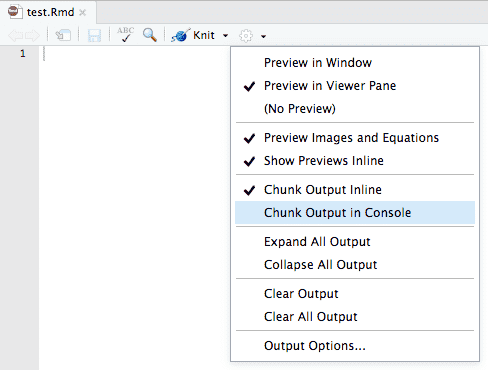
By default, RStudio enables inline output (Notebook mode) on all R Markdown documents. This means that if you run a code chunk in R markdown on R studio, all the output, including the figure, is displayed below the end of the code chunk you just run (See the picture below). While this feature lets you interact with any R Markdown like a notebook, sometimes it is inconvenient, especially if you have a large code chunk. You can turn off this feature and display the code output in the console pane like in the usual R script (I had been bothered for long time until I found this solution.) Go to the gear button in the editor toolbar, and choose “Chunk Output in Console.” You will see that the chunk_output_type option is added to the YAML header of your R Markdown document.

editor_options:
  chunk_output_type: console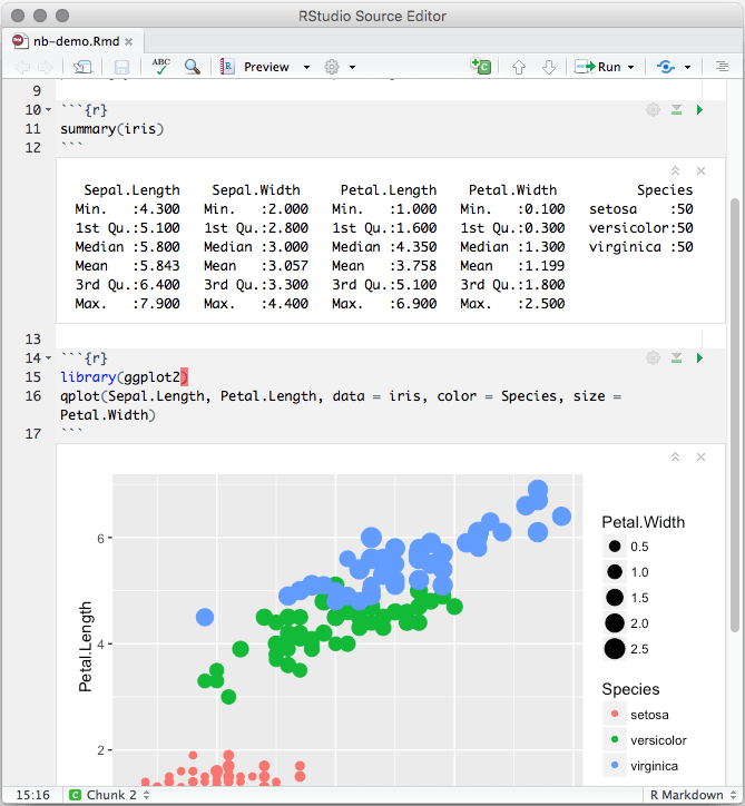

Notebook mode (Default)
How to disable Notebook mode?

Rmarkdown: inline output (Notebook mode)

Choose “Chunk Output in Console”.

How to disable inline output (Notebook mode)

Reference: Section 3.2 Notebook in “R Markdown: The Definitive Guide” by Yihui Xie, J. J. Allaire, Garrett Grolemund

3. Summary

I hope you now have a better understanding of how to use Rmarkdown. The trickiest part might be setting up the YAML header and code chunk options. But don’t worry! You can always start with a template and modify it to fit your needs.
Check this official website for Rmarkdown for more detailed information: R Markdown Introduction.

Footnotes

output: pdf_document, output: html_document, and output: word_document can be used for simple documents, but you have better output options from bookdown (Xie, 2024), which is an R Markdown extension. For example, use output: bookdown::bookdown::pdf_document2 to create a PDF document. This option lets you use advanced functionalities such as cross-referencing for equations, tables, and figures.↩︎
Cross-referencing is not provided directly within the base rmarkdown package, but is provided as an extension in bookdown (Xie 2023a). For further information, see this document this document ↩︎